Google Kubernetes Engine (GKE) is the default Kubernetes platform for many production teams. This managed service lets Google provision and operate the underlying infrastructure and Kubernetes control plane, while you define the clusters, workloads, and policies that control how containers are deployed, scaled, and managed.
But as GKE adoption has matured, a major (and growing) problem has followed: cloud waste. A 2025 study found that 30% of enterprise cloud spending is addressable waste. So what should you be doing?
GKE cost optimization isn’t just about “saving money.” It’s about eliminating waste and getting more value from what you already pay for: compute, cluster configuration, autoscaling, storage, network traffic, load balancers, and observability (logs and metrics).
In this article, we’ll spend less time explaining how GKE works and more time on how strong teams optimize it in the real world—where manual tuning doesn’t scale, waste slowly returns, and cost efficiency becomes a continuous discipline, not a one-time project.
Where Manual GKE Cost Optimization Breaks Down
Most teams can find quick wins in the first few weeks. They tighten requests, tune autoscaling, and buy some discounts. The problem is that GKE environments don’t stay still. As teams grow, the gap between “we optimized once” and “we’re optimized now” widens quickly.
Here are the most common failure modes we see when optimization stays manual:
- Configuration drift: Workload owners change requests/limits, new services launch, and yesterday’s rightsizing assumptions quietly expire.
- Policy trade-offs at scale: You can’t have every workload perfectly tuned for cost, latency, and reliability at all times, and manual processes force compromises that revert to overprovisioning.
- Discount leakage: Teams commit CUDs off inflated baselines, then can’t keep utilization high, resulting in discounted capacity sitting idle while spikes spill into on-demand.
- Autoscaling without guardrails: HPA/Cluster Autoscaler settings get tuned for peak safety, but downscaling becomes conservative, leaving “always-on headroom” that turns into permanent waste.
- No clear ownership: Platform teams see the bill, app teams control specs. Without continuous feedback loops, waste becomes a coordination problem.
ScaleOps fits naturally with GKE by autonomously managing resources across the cluster, from pod requests/limits to node capacity. It continuously rightsizes workloads and keeps scaling behavior healthy over time, so clusters stay efficient without constant manual tuning. As a result, teams reduce waste while staying aligned with commitments like CUDs and avoiding unnecessary spillover into on-demand.
Understanding GKE Pricing
GKE is managed Kubernetes. Google runs the control plane while your workloads run on the data plane.
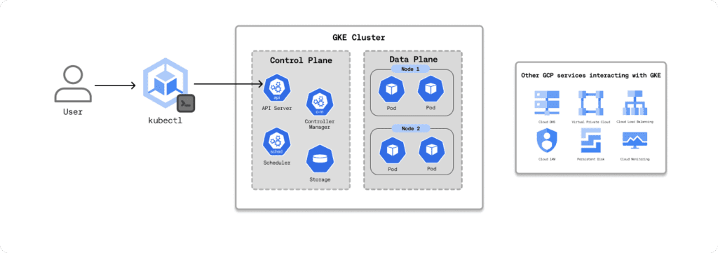
From a billing perspective, it helps to break a GKE cluster into three cost buckets:
- Control plane and cluster management
- Data plane compute and storage (your worker nodes and persistent volumes)
- Other GCP services the cluster depends on (for example load balancing, networking, and observability)
Let’s start with the GKE free tier, then move on to the main cost drivers.
GKE Free Tier
GKE’s free tier is part of Google Cloud’s Always Free offering, so it applies to both new and existing accounts and renews every month. Each billing account gets $74.40/month in GKE credits that can be applied to the cluster management fee, enough to cover roughly one Autopilot cluster or one zonal Standard cluster running continuously for a month.
| (Flat cluster management fee/hr) * (hrs/month) | Monthly cluster management fee |
| $0.1 * 744 | $74.40 |
Important: the free tier only applies to the management fee. You still pay for the resources your workloads consume, worker nodes, storage, and any other GCP services the cluster uses (for example load balancers, logging/monitoring, and network egress).
Control Plane and Cluster Management Costs
GKE charges a flat cluster management fee of $0.10 per cluster-hour (billed in one-second increments). The rate is the same whether the cluster is zonal, regional, multi-zonal, or Autopilot.
That fee covers the managed Kubernetes control plane, API server, scheduler, controllers, and etcd, plus the compute and storage Google runs it on. You don’t size or pay for the control plane’s underlying VMs and disks directly; they’re included in the management fee.
Data Plane Compute and Storage Cost
GKE data plane costs depend on how you provision compute. You have two options: Standard mode or Autopilot mode.
Standard Mode
In Standard mode, you manage the nodes yourself. You create node pools backed by Compute Engine VMs and choose the machine type, disk size, and any accelerators. Compute Engine VMs used as GKE nodes are billed per second, with a one-minute minimum.
The pricing model is straightforward: allocated node capacity equals your bill. If you overprovision nodes, or if Pods do not pack efficiently, you pay for unused capacity. Upgrade headroom and disruption budgets can also keep extra nodes running and increase spend.
Autopilot Mode
In Autopilot mode, Google manages the nodes for you. You are billed based on what your Pods request, not the node capacity. Charges accrue per second for vCPU, memory, and ephemeral storage for Pods in Running and ContainerCreating states.
As of early 2026, general-purpose Autopilot pricing in us-central1 is about $0.0445 per vCPU-hour, $0.0049 per GiB-hour of memory, and $0.00014 per GiB-hour of ephemeral SSD storage. Prices vary by region and discount programs may apply.
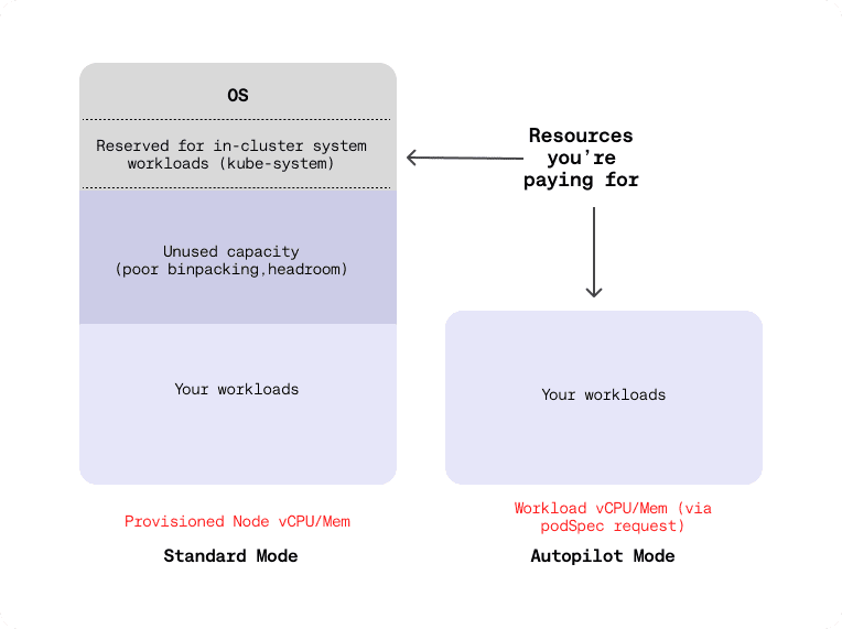
Standard mode vs. Autopilot mode (Adapted from Google Cloud)
In Autopilot, Pod resource requests are effectively your bill. Overstated CPU and memory requests show up as direct waste. Autopilot is attractive for speed and operational simplicity, but cost tuning depends on teams setting accurate requests and sane scaling policies.
Some operations teams avoid the default Autopilot billing behavior by using a custom ComputeClass so pricing aligns more closely with the underlying hardware profile.
Operational takeaway
The biggest ongoing cost lever is automated workload rightsizing. Continuously manage pod CPU and memory requests and review autoscaling behavior based on real usage.
Other Services GKE Interacts With
On top of control plane and data plane costs, teams also pay for the Google Cloud services that sit around GKE, allowing an application to function:
- Networking and traffic handling: VPC, cloud load balancing, Cloud NAT, Cloud DNS
- Image and configuration supply chain: Artifact Registry, Secret Manager
- Observability: Cloud Logging, Cloud Monitoring
Each of these is billed under its own stock-keeping unit (SKU), often contributing as much to the monthly bill as the cluster compute itself.
Some GKE features are billed as standalone SKUs, such as Multi Cluster Gateway and Multi Cluster Ingress, Backup for GKE, extended support, and hybrid and multi-cloud. Fees for these features only show up on the bill if you enable them.
Best Practices for GKE Cost Optimization
When managing GKE costs, the goal isn’t to minimize usage at all costs. Instead, focus on making informed optimization decisions that reduce waste without compromising application reliability or the end-user experience.
Google defines four “golden signals” for Kubernetes cost optimization in public cloud environments:
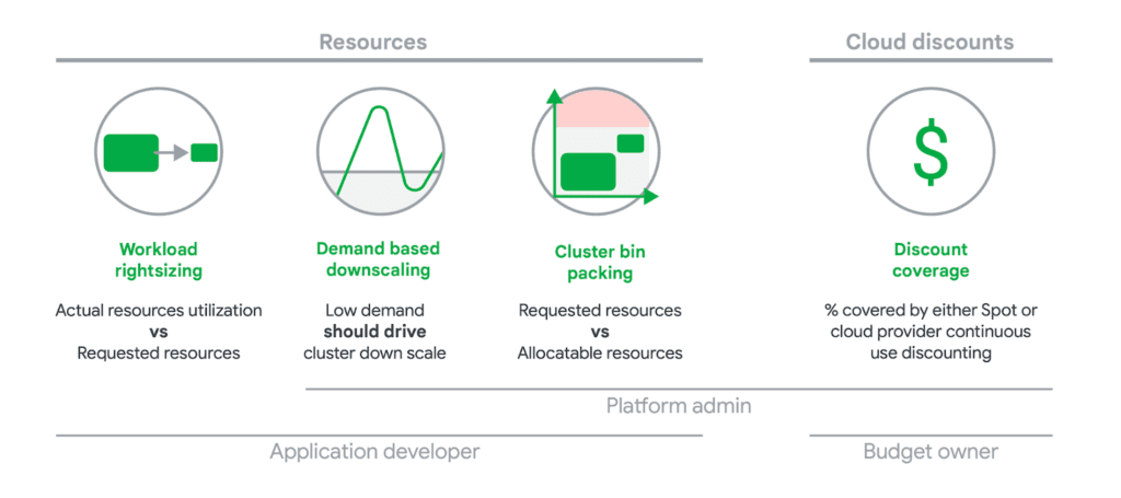
Building on these principles and our hands-on experience working with GKE environments at ScaleOps, here is an actionable, practical checklist for optimizing your GKE costs effectively.
New Spend-Based Committed Use Discounts (CUDs)
Spend-based/flexible CUDs are 1-year or 3-year commitments for a lower rate versus on-demand pricing:
- A 1-year term results in a 28% discount from your committed hourly spend.
- A 3-year term results in a 46% discount from your committed hourly spend.
From January 2026, Google will have fully migrated customers to this new model. These commitments are not tied to a specific machine type; instead, they are based on a minimum hourly spend on eligible resources such as vCPU, memory, and ephemeral storage across both Standard and Autopilot mode.
Scenario
- Two GKE Autopilot clusters
- Regions: us-central1 (Iowa) and me-central1 (Doha)
- Workload per region: 4 vCPUs + 6 GB memory
- Commitment type: 1-year Committed Use Discount (28%)
Monthly & hourly costs with 1-year CUD
| Region | Hourly Cost (vCPU) | Hourly Cost (Memory) | Total / Hour | Total / Month |
| Iowa | $0.1281 | $0.0213 | $0.1494 | $109.06 |
| Doha | $0.1558 | $0.0258 | $0.1816 | $132.57 |
| Total | — | — | $0.3310 | $241.63 |
💡 Monthly costs assume 730 hours.
Baseline cost (No commitment)
| Region | Total / Hour | Total / Month |
| Iowa | $0.2075 | $155.63 |
| Doha | $0.2522 | $184.11 |
Monthly savings with 1-year CUD
| Region | Baseline | With CUD | Monthly Savings |
| Iowa | $155.63 | $109.06 | $46.56 |
| Doha | $184.11 | $132.57 | $51.54 |
| Total | — | — | $98.10/month |
A 1-year CUD for this Autopilot workload saves ~$98/month, or ~$1,177 per year, across two regions, without changing a single pod configuration.
As shown above, Committed Use Discounts (CUDs) are one of the most underrated differentiators between elite and low-performing cloud cost optimization teams. When used correctly, they deliver predictable, material savings. When used poorly, they simply lock in inefficiency.
The key tradeoff is commitment: once you purchase a CUD, you’re locked into that spend for the full term. That’s why the order of operations matters.
Optimize before you commit
A common mistake is purchasing CUDs based on current usage, which is almost always overprovisioned. While this technically reduces your bill, it does so by discounting waste, not eliminating it.
The better approach is:
- Rightsize workloads first to establish a lean, stable baseline
- Then purchase CUDs against that optimized footprint
This ensures your commitments are tied to real, sustained demand—not temporary spikes or historical misconfigurations.
How ScaleOps Maximizes CUD ROI
ScaleOps maximizes ROI by continuously rightsizing workloads to actual usage, not static assumptions. By integrating directly with GCP Billing, ScaleOps enables teams:
- Optimize resource allocation within committed spend
- Free up discounted capacity for new workloads
- Avoid wasting CUDs on underutilized or idle resources
The result: commitments stay fully utilized, and discounted capacity is treated as a strategic asset, not a sunk cost.
Discounted Spot VMs
Spot VMs provide access to deeply discounted Compute Engine capacity, with the tradeoff of reduced availability. These instances are built from spare regional capacity and can be reclaimed by Google at any time when higher-priority demand arises.
Because of their ephemeral nature, Spot VMs are best suited for batch, stateless, or fault-tolerant workloads. When used correctly, they can deliver dramatic savings—sometimes up to 91% off the standard on-demand price.
Google-Recommended Best Practice for Spot VMs
Google recommends a hybrid approach to balance cost and reliability:
- Maintain a backup node pool with regular (non-Spot) VMs
- Configure Cluster Autoscaler to scale Spot nodes first
- Allow the cluster to fall back to standard nodes when Spot capacity is unavailable
To protect critical workloads, use taints and tolerations to ensure system components (like DNS) and latency-sensitive services never land on Spot nodes.
This approach lets you aggressively capture Spot savings without putting cluster stability at risk.
Fine-Tuned GKE Autoscaling
Autoscaling is the third major cost lever after discount coverage from CUDs and Spot capacity. In practice, autoscaling does two things:
- Keeps workloads and infrastructure rightsized for real demand
- Performs demand-based downscaling so idle capacity gets removed instead of sitting around unused
The GKE autoscaling stack has four dimensions. In Standard mode, you own the autoscaling stack end-to-end, whereas in Autopilot mode, you only tune scaling at the workload layer.
Essentially, autoscaling is how you turn Kubernetes elasticity into “only pay for what you actually use” instead of carrying static headroom.
But fine-tuning it is not as easy as it sounds. Start be referencing Google’s GKE optimizations best practices:
- Ensure the application boots fast and exits gracefully according to Kubernetes expectations (graceful termination,
preStophooks,terminationGracePeriod). - Set meaningful readiness and liveness probes so load balancers only send traffic to truly ready pods.
- Define Pod disruption budgets (PDBs) for your applications so CA can evict Pods safely without breaking availability.
- Use HPA for sudden or unpredictable spikes; base it on CPU, memory, or custom metrics that actually reflect load.
- Use either HPA or VPA to autoscale a given workload (not both on the same metric) to avoid oscillation/thrashing.
- Be sure that your Metrics Server remains available.
- Run short-lived or easily restarted Pods in separate node pools so long-lived Pods don’t block node scale-down decisions.
- Configure pause Pods to handle short spikes.
Native Kubernetes prevents you from using HPA and VPA on the same metric, which often forces teams to choose between rightsizing (VPA) and scaling out (HPA). This is where ScaleOps differs from the GKE Standard: It automates workload rightsizing while respecting billing commitments and CUDs, helping ensure you don’t scale into expensive on-demand usage unnecessarily.
Choosing the Right Machine Types
E2 VMs are cost-optimized and can be roughly 30% cheaper than older N1 types, while still suitable for most environments. From there, you can move up to more expensive families (N2, N2D, Tau, GPU nodes) only when you have a measured need.
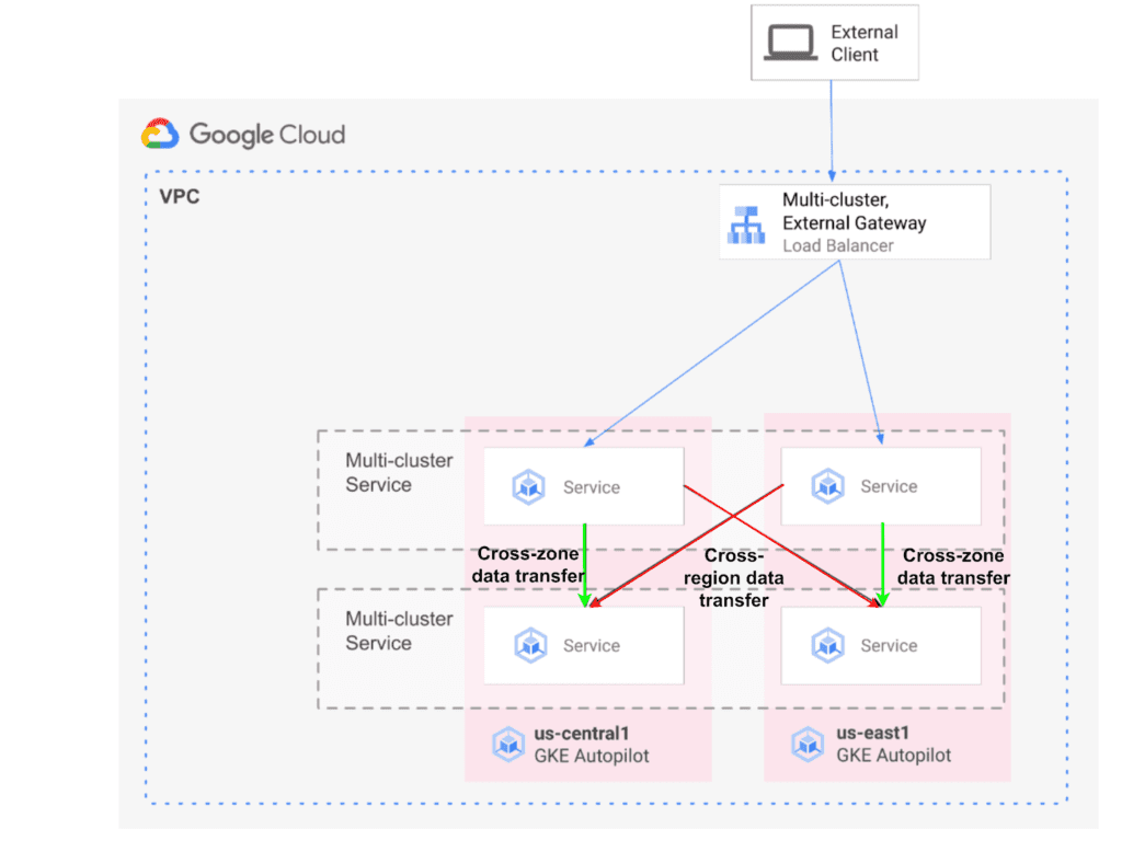
Cross-Region and Cross-Zone Data Transfer
There are three types of GKE clusters: single-zone, multi-zonal, and regional. From a cost standpoint, the main difference is how much cross-zone and cross-region traffic you generate.
Single-zone clusters keep all nodes in one zone, the trade-off being availability.
Multi-zonal and regional clusters spread nodes across zones in the same region, offering high availability. However, if chatty services are spread across zones, the “cross-zone data transfer” SKU will add up inside that region.
For example, the podAntiAffinity rule below forces each payments-api Pod onto a different zone in the region, preventing multiple replicas from running in the same zone:
spec:
  template:
    metadata:
      labels:
        app: payments-api
    spec:
      affinity:
        podAntiAffinity:
          requiredDuringSchedulingIgnoredDuringExecution:
          - labelSelector:
              matchLabels:
                app: payments-api
            topologyKey: topology.kubernetes.io/zone
Moreover, any traffic that leaves a region is billed as inter-region network egress, which can quickly become a hidden cost driver. For this reason, the default strategy should be to run clusters in the lowest-cost region possible and avoid moving data across regions unless there is a clear technical or business requirement (such as latency, compliance, or resilience).
As a starting point, Google’s Compute Engine region selection guide provides a solid framework for evaluating regional tradeoffs around cost, latency, and availability.
Cluster Bin Packing
While cluster autoscaling decides how many nodes you run, cluster bin packing decides how full those nodes actually are. Poor bin packing strands small chunks of CPU and memory on a node, which forces CA or Autopilot mode to add more nodes even when there is enough raw capacity.
In practice, good bin packing comes down to a few rules:
- Standardize on node pool shapes whose CPU-to-memory ratio matches the Pod profile.
- Reserve taints or dedicated node pools for the minority of workloads that really need isolation.
- Avoid unnecessary nodeSelector and hard podAntiAffinity rules; use preferredDuringSchedulingIgnoredDuringExecution so the scheduler can pack efficiently.
Observability and Automation
It’s the developer’s responsibility to make sure best practices are in place. But perfect systems do not exist, and in the end, cost optimization boils down to observability.
As a starting point, the GKE console exposes charts for metrics such as CPU and memory request utilization, cAdvisor metrics, startup latency, and many others. On top of that, GKE usage metering breaks down usage by namespace and labels, making it clear which teams and workloads are driving most of the GKE spend.
Native GKE and Cloud Monitoring tools are great at telling what’s happening, but they stop at observability without taking action on those insights. That’s why there are tools like ScaleOps that consume this resource telemetry and turn it into concrete changes for optimization.
Cloud Resource Management Is All You Need: ScaleOps
GKE cost optimization isn’t a one-time cleanup. It requires visibility across all namespaces and workloads, plus automation to keep resources rightsized as things change. The goal isn’t one-off tweaks or “set and forget” configs, but continuous optimization in production that stays accurate over time.
ScaleOps supports this shift as a cloud resource management platform. It runs inside your clusters and provides context-aware, application-aware, real-time automated Pod rightsizing, with cost savings as a natural by-product of that automation. Most importantly, it automates cost optimization while maximizing both performance and reliability.
Run GKE lean, without turning your team into full-time cost-tuners. Book a demo of ScaleOps today.